Cycle closure: what it measures and what it cannot
Relative binding free energy (RBFE) calculations use molecular dynamics simulations to determine the free energy difference \(\Delta\Delta G\) between ligands, from which absolute binding free energy \(\Delta G\) can be derived (up to an overall constant). The ligands and the simulated pairs form a graph: ligands are nodes, and each measurement (calculation) is an edge.
A classic sanity check on such data is cycle closure: pick a closed loop of edges, say \(A\to B\to C\to A\), and add up the measured \(\Delta\Delta G\)’s with signs. Since free energy is a state function, the exact values must sum to zero; whatever is left over is error. It feels like a free lunch — no experimental data is needed, and any non-zero closure is a smoking gun.
In this post I will work out precisely what cycle closure measures, using little more than linear algebra. The punchline is that closure sees only part of the error, and the part it cannot see is often the part you care about.
Contents
- the model
- splitting the ΔΔG data in two
- case 1: ordinary least squares (OLS)
- case 2: weighted least squares (WLS)
- leaving one edge out
- never make closure the objective
- what closure cannot see
- summary
- appendix: try it yourself
the model
Stack the \(n\) unknown per-ligand free energies into \(\mathbf x\in\mathbb R^n\) and the \(m\) measured edge values into \(\mathbf y\in\mathbb R^m\). An edge measuring the pair \(a\to b\) ideally reports \(x_b - x_a\), so
\[\mathbf y = \mathbf B \mathbf x + \boldsymbol\epsilon\]where \(\mathbf B\) is the \(m\times n\) signed incidence matrix: the row for edge \(a\to b\) has \(-1\) in column \(a\), \(+1\) in column \(b\), and zeros elsewhere. This is a plain linear regression, except the design matrix is special: every row is a difference of two node indicators, \(\mathbf b_i = \mathbf e_b - \mathbf e_a\). In other words, \(\mathbf B\) is the discrete gradient on the graph.
For the noise \(\boldsymbol\epsilon\), I will assume as little as possible for now — a mean and a covariance, no distributional shape:
\[\mathbb E[\boldsymbol\epsilon] = \mathbf 0, \qquad \mathrm{Cov}(\boldsymbol\epsilon) = \boldsymbol\Sigma \ \text{(unknown)}\]Since \(\mathbf x\) is a fixed unknown, the covariance of the data is simply
\[\mathrm{Cov}(\mathbf y) = \boldsymbol\Sigma\]two structural facts, before any statistics
The incidence structure gives two facts for free, valid for any noise model.
1. A global offset is unobservable. Every row of \(\mathbf B\) sums to zero, so \(\mathbf B\mathbf 1 = \mathbf 0\): adding a constant to every ligand’s free energy changes no edge difference. For a connected graph this is the only degeneracy, \(\mathrm{rank}(\mathbf B) = n-1\), and \(\mathbf x\) is identifiable only up to an additive constant (a gauge freedom). This is physically sensible — relative measurements can never fix an absolute scale.
2. Cycles annihilate the signal. Let \(\mathbf z\in\mathbb R^m\) be a cycle indicator: \(\pm 1\) on the edges of a closed loop (sign tracking direction), zero elsewhere. Walking around the loop, each node is entered once and left once, so the node contributions cancel:
\[\mathbf z^\mathsf T \mathbf B = \mathbf 0\]The set of all such vectors (and their linear combinations) is the cycle space, the orthogonal complement of \(\mathrm{col}(\mathbf B)\), the left null space of \(\mathbf B\), with dimension \(m - n + 1\) for a connected graph. Applying \(\mathbf z\) to the model,
\[C(\mathbf z) \equiv \mathbf z^\mathsf T\mathbf y = \mathbf z^\mathsf T\mathbf B\mathbf x + \mathbf z^\mathsf T\boldsymbol\epsilon = \mathbf z^\mathsf T\boldsymbol\epsilon\]The closure error is pure noise: the true free energies drop out identically. This is both the charm and the curse of cycle closure.
- The charm: closure needs no reference values, experimental or otherwise — it is a property of the measurements alone.
- The curse: it can only ever see the component of \(\boldsymbol\epsilon\) that lives in the cycle space.
As a warm-up with numbers, a triangle with measurements \(y_{AB}=0.5\), \(y_{BC}=-1.2\), \(y_{CA}=0.8\) (kcal/mol) has closure \(C = 0.5 - 1.2 + 0.8 = 0.1\), and no assignment of per-ligand values can absorb it. Hold that thought.
least squares and the covariance of the estimate
To turn \(m\) edge measurements into \(n\) ligand values, we solve a least-squares problem. Allow a generic symmetric positive definite weight \(\mathbf W\) for now:
\[\hat{\mathbf x} = \arg\min_{\mathbf x}\; (\mathbf y - \mathbf B\mathbf x)^\mathsf T \mathbf W (\mathbf y - \mathbf B\mathbf x)\]It is worth being clear about what \(\mathbf W\) is. It is our model of the noise — a statement about which edges we believe more, entered by hand before any fitting happens. It is NOT the covariance \(\boldsymbol\Sigma\) above: \(\boldsymbol\Sigma\) is a fact about the world, fixed and unknown, while \(\mathbf W\) is a choice we make and can get wrong. The natural choice is \(\mathbf W = \boldsymbol\Sigma^{-1}\) — trust each edge in inverse proportion to its variance — but nothing enforces that, and keeping the two symbols apart allows us to ask later what happens when the noise model is wrong.
Why this objective, and why those weights? For Gaussian noise it is exactly the maximum-likelihood estimator, since \(-\log P(\mathbf y\mid\mathbf x)\) is this weighted sum of squares, see my earlier post on maximum likelihood and maximum a posteriori methods.
The normal equation is \(\mathbf B^\mathsf T\mathbf W\mathbf B\, \hat{\mathbf x} = \mathbf B^\mathsf T\mathbf W\mathbf y\). Define
\[\mathbf L = \mathbf B^\mathsf T\mathbf W\mathbf B\]For diagonal \(\mathbf W\) this is the weighted graph Laplacian — the same matrix that appears in circuit theory and spectral graph theory. Writing the sum over edges,
\[\mathbf L = \sum_i w_i\,\mathbf b_i\mathbf b_i^\mathsf T = \sum_{(a,b)} w_{ab}(\mathbf e_b - \mathbf e_a)(\mathbf e_b - \mathbf e_a)^\mathsf T\]Each edge contributes \(+w_{ab}\) to the two diagonal entries \((a,a)\) and \((b,b)\), and \(-w_{ab}\) to the two off-diagonal entries \((a,b)\) and \((b,a)\). Summing over edges,
\[\mathbf L = \mathbf D - \mathbf A\]where \(\mathbf A\) is the weighted adjacency matrix (\(A_{ab} = w_{ab}\) if \(a\sim b\), else 0) and \(\mathbf D\) is the diagonal weighted degree matrix, \(D_{aa} = \sum_b w_{ab}\). This form makes two things immediate. Each row sums to zero, which is the gauge \(\mathbf L\mathbf 1 = \mathbf 0\) again; and \(\mathbf L\) depends only on the undirected weighted graph — the sign convention that oriented each edge has vanished. In the unweighted case (\(\mathbf W = \mathbf I\)) this is the plain graph Laplacian \(\mathbf L = \mathbf D - \mathbf A\) with \(D_{aa}\) the plain node degree — the number of edges touching ligand \(a\).
Because \(\mathbf L\) is singular (\(\mathbf L\mathbf 1 = \mathbf 0\), the gauge again), the solution uses the pseudo-inverse:
\[\hat{\mathbf x} = \mathbf L^{+}\mathbf B^\mathsf T\mathbf W\,\mathbf y\]The pseudo-inverse picks the minimum-norm solution, which is mean-centered — a convention for the gauge, nothing more. Taking expectations, \(\mathbb E[\hat{\mathbf x}] = \mathbf L^{+}\mathbf L\,\mathbf x\), which is \(\mathbf x\) with its mean subtracted: the estimate is unbiased up to the unobservable constant.
Now the covariance. Since \(\hat{\mathbf x}\) is linear in \(\mathbf y\),
\[\mathrm{Cov}(\hat{\mathbf x}) = \mathbf L^{+}\mathbf B^\mathsf T\mathbf W\, \boldsymbol\Sigma\, \mathbf W\mathbf B\,\mathbf L^{+}\]This “sandwich” form is exact for any noise covariance \(\boldsymbol\Sigma\) and any weight choice \(\mathbf W\) — the model and the world need not agree. Most of what follows assumes they do agree; what closure cannot see is what happens when they do not.
splitting the ΔΔG data in two
The fitted edge values are \(\hat{\mathbf y} = \mathbf B\hat{\mathbf x} = \mathbf H\mathbf y\), where
\[\mathbf H = \mathbf B\mathbf L^{+}\mathbf B^\mathsf T\mathbf W\]is the hat matrix (it puts the hat on \(\mathbf y\)). It is idempotent, \(\mathbf H^2 = \mathbf H\), which follows from \(\mathbf L^{+}\mathbf L\mathbf L^{+} = \mathbf L^{+}\) — so it is a projection, and the whole analysis is the trivial identity (writing \(\tilde{\boldsymbol\epsilon}\) for the residual):
\[\boxed{\; \mathbf y = \underbrace{\mathbf H\mathbf y}_{\text{explainable}} + \underbrace{(\mathbf I - \mathbf H)\mathbf y}_{\text{closure error}} \;=\; \hat{\mathbf y} + \tilde{\boldsymbol\epsilon} \;}\]This one line is the whole post in miniature. Least squares splits the \(m\) measurements into two pieces that live in complementary subspaces of \(\mathbb R^m\), and every statement below is about which piece a given diagnostic can see.
- \(\mathbf H\mathbf y\) lands in \(\mathrm{col}(\mathbf B)\), dimension \(n-1\). This is the part expressible as differences of per-ligand numbers — the part a set of \(\Delta G\)’s can account for.
- \((\mathbf I-\mathbf H)\mathbf y\) lands in \(\ker(\mathbf B^\mathsf T\mathbf W)\), dimension \(m-n+1\). This is what no assignment of per-ligand numbers can produce.
The split is orthogonal in the \(\mathbf W\) inner product \(\langle \mathbf u,\mathbf v\rangle_{\mathbf W} = \mathbf u^\mathsf T\mathbf W\mathbf v\) (for OLS, \(\mathbf W = \mathbf I\), ordinary orthogonality), which is just least squares doing its job: it removes as much of \(\mathbf y\) as the model can reach, leaving a remainder the model cannot touch. Two consequences follow. Since \((\mathbf I - \mathbf H)\mathbf B = \mathbf 0\), the residual is blind to \(\mathbf x\) exactly as the loop sums are — indeed the loop sums are simply particular coordinates of \((\mathbf I-\mathbf H)\mathbf y\). And both halves carry covariances of the same shape. Each is a linear map applied to \(\mathbf y\), so each covariance is \(\boldsymbol\Sigma\) sandwiched between that map and its transpose:
\[\mathrm{Cov}(\hat{\mathbf x}) = \mathbf L^{+}\mathbf B^\mathsf T\mathbf W\,\boldsymbol\Sigma\,\mathbf W\mathbf B\mathbf L^{+}, \qquad \mathrm{Cov}(\tilde{\boldsymbol\epsilon}) = (\mathbf I - \mathbf H)\,\boldsymbol\Sigma\,(\mathbf I - \mathbf H)^\mathsf T\]The first is the sandwich from the previous section, now readable as what it is: the fitted half \(\mathbf H\mathbf y\) carried through to ligand space.
Both collapse the moment the weights match the noise, \(\boldsymbol\Sigma = \mathbf W^{-1}\):
\[\mathrm{Cov}(\hat{\mathbf x}) = \mathbf L^{+}, \qquad \mathrm{Cov}(\tilde{\boldsymbol\epsilon}) = (\mathbf I - \mathbf H)\mathbf W^{-1} = \mathbf W^{-1} - \mathbf B\mathbf L^{+}\mathbf B^\mathsf T\]The first because \(\mathbf W\boldsymbol\Sigma\mathbf W = \mathbf W\) turns the sandwich into \(\mathbf L^{+}\mathbf L\mathbf L^{+} = \mathbf L^{+}\); the second because \((\mathbf I-\mathbf H)\mathbf B = \mathbf 0\) annihilates the trailing factor. So under the right weights the covariance of the answer is simply the pseudo-inverse of the Laplacian.
One more fact about the pair, worth having before we go on. Under the same \(\boldsymbol\Sigma = \mathbf W^{-1}\), the cross-covariance collapses too:
\[\mathrm{Cov}(\hat{\mathbf x},\,\tilde{\boldsymbol\epsilon}) = \mathbf L^{+}\mathbf B^\mathsf T\mathbf W\,\boldsymbol\Sigma\,(\mathbf I-\mathbf H)^\mathsf T = \mathbf L^{+}\big[(\mathbf I-\mathbf H)\mathbf B\big]^\mathsf T = \mathbf 0\]The answer and the closure error are uncorrelated — exactly, not approximately, when the noise model is right. Whatever the residual happens to do on a given dataset, it carries no information about how far that dataset’s \(\hat{\mathbf x}\) has strayed.
the two subspaces, and their many names
These two subspaces get different names in linear algebra, in graph theory, in physics, and in statistics:
| fitted part \(\mathbf H\mathbf y\) | residual part \((\mathbf I-\mathbf H)\mathbf y\) | |
|---|---|---|
| linear algebra | column space \(\mathrm{col}(\mathbf B)\) | its \(\mathbf W\)-orthogonal complement, \(\ker(\mathbf B^\mathsf T\mathbf W)\) |
| graph theory | cut space (cocycle, bond space) | cycle space (circuit, flow space) |
| vector calculus | gradient field | divergence-free circulation |
| circuits | potential drops (KVL) | loop currents |
| statistics | fitted values | residuals |
| this problem | differences of per-ligand \(\Delta G\) | cycle-closure error |
| dimension | \(n - 1\) | \(m - n + 1\) |
| spanned by | the \(n-1\) independent cuts | the \(m-n+1\) independent loops |
The vector-calculus row is not a loose analogy: the split \(\mathbf y = \mathbf B\hat{\mathbf x} + \tilde{\boldsymbol\epsilon}\) is the discrete Helmholtz–Hodge decomposition of an edge flow into a gradient plus a circulation, with \(\mathbf B\) the discrete gradient and \(\mathbf B^\mathsf T\mathbf W\) the discrete divergence.
One point of precision is worth making, since this is easy to get wrong and the right version is prettier. The graph-theoretic cycle space is \(\mathcal C = \ker(\mathbf B^\mathsf T) = \{\mathbf z : \mathbf B^\mathsf T\mathbf z = \mathbf 0\}\), the circulations. The residual lives in \(\ker(\mathbf B^\mathsf T\mathbf W) = \mathbf W^{-1}\mathcal C\), which is the same space only when \(\mathbf W \propto \mathbf I\). What is a genuine circulation for any \(\mathbf W\) is \(\mathbf W\tilde{\boldsymbol\epsilon}\) — the vector of currents, since \(\mathbf B^\mathsf T(\mathbf W\tilde{\boldsymbol\epsilon}) = \mathbf 0\). So the “cycle space” column above is exact for OLS and, for weighted fits, is the space the currents live in. None of this touches the closure sums themselves: \(\mathbf z^\mathsf T\mathbf y = \mathbf z^\mathsf T\tilde{\boldsymbol\epsilon}\) for every \(\mathbf z\in\mathcal C\) and every \(\mathbf W\), because \(\mathbf z^\mathsf T\mathbf B = \mathbf 0\) does the work by itself.
A warning about the name. “Cycle space” does not mean “sums to zero around every cycle” — it means the exact opposite, and the two conditions belong to the two different columns above.
test \(\mathbf H\mathbf y\) (cut space) \(\tilde{\boldsymbol\epsilon}\) (cycle space) signed sum around every loop \(0\) not \(0\) net current at every node (weighted divergence) not \(0\) \(\mathbf 0\) The residual’s currents sum to zero at every ligand, not around every loop — that vanishing divergence is precisely the normal equations \(\mathbf B^\mathsf T\mathbf W\tilde{\boldsymbol\epsilon} = \mathbf 0\), which we will meet again as Kirchhoff’s current law. (For OLS the weights are \(1\) and this is the plain signed sum.) The space is called the cycle space because it is spanned by loop circulations — the \(\pm 1\) vectors \(\mathbf z\) from before — and each of those is individually divergence-free.
case 1: ordinary least squares (OLS)
The simplest assumption: all edges are equally noisy and independent,
\[\boldsymbol\Sigma = \sigma^2\mathbf I, \qquad \mathbf W = \mathbf I\]The sandwich collapses, \(\mathbf L^{+}\mathbf B^\mathsf T \sigma^2\mathbf I\, \mathbf B \mathbf L^{+} = \sigma^2\mathbf L^{+}\mathbf L\mathbf L^{+}\), giving
\[\mathrm{Cov}(\hat{\mathbf x}) = \sigma^2\,\mathbf L^{+}, \qquad \mathbf L = \mathbf B^\mathsf T\mathbf B\]the pseudo-inverse of the plain (unweighted) graph Laplacian. The variance of a difference — the only gauge-invariant quantity — is
\[\mathrm{Var}(\hat x_b - \hat x_a) = \sigma^2 (\mathbf e_b-\mathbf e_a)^\mathsf T \mathbf L^{+} (\mathbf e_b-\mathbf e_a) = \sigma^2 R_{\mathrm{eff}}(a,b)\]where \(R_{\mathrm{eff}}\) is the effective resistance between the two nodes when every edge is a \(1\,\Omega\) resistor. This single identity carries all the design intuition: edges in series add resistance (long chains of ligands accumulate variance), edges in parallel reduce it (redundant paths average noise down), and a bridge — an edge in no cycle — contributes its full resistance, uncheckable by any closure.
The noise assumption also fixes the statistics of closure itself. For a single loop of length \(\ell\),
\[\mathrm{Var}\big(C(\mathbf z)\big) = \mathbf z^\mathsf T\boldsymbol\Sigma\,\mathbf z = \sigma^2\|\mathbf z\|^2 = \sigma^2 \ell\]so closure errors of honest, independent noise grow as \(\sqrt{\ell}\). This is a useful diagnostic in its own right: if observed closures are flat in cycle length, the error is not diffuse noise but is concentrated on a few bad edges — the loop sum is dominated by whichever bad edge it contains.
And the residual gives an estimate of \(\sigma\) for free. With \(\mathrm{Cov}(\tilde{\boldsymbol\epsilon}) = \sigma^2(\mathbf I - \mathbf H)\) and \(\mathrm{tr}(\mathbf I - \mathbf H) = m - n + 1\),
\[\mathbb E\left[\|\tilde{\boldsymbol\epsilon}\|^2\right] = \sigma^2\,(m-n+1)\]The number of degrees of freedom is the dimension of the cycle space — the number of independent loops. A spanning tree has \(m = n-1\): zero degrees of freedom, residual identically zero, nothing to check. Redundancy is what buys testability.
case 2: weighted least squares (WLS)
In practice edges are not equally noisy: each edge comes with its own error bar \(\sigma_i\) (from the BAR estimator or from replicates). The natural model and the natural weights are
\[\boldsymbol\Sigma = \mathrm{diag}(\sigma_i^2), \qquad \mathbf W = \boldsymbol\Sigma^{-1}\]This is the \(\boldsymbol\Sigma = \mathbf W^{-1}\) case already met when we split the data, so \(\mathrm{Cov}(\hat{\mathbf x}) = \mathbf L^{+}\) carries over unchanged. What is new is that the weights are now concrete, and \(\mathbf L\) becomes a sum over edges:
\[\mathbf L = \mathbf B^\mathsf T\mathbf W\mathbf B = \sum_i \frac{\mathbf b_i\mathbf b_i^\mathsf T}{\sigma_i^2}\]each edge contributing in inverse proportion to its variance. These are also the maximum-likelihood weights, by the derivation cited earlier. By the Gauss–Markov theorem in Aitken’s generalized form, this choice is optimal — minimum variance among all linear unbiased estimators of the ligand differences (the gauge-invariant quantities; \(\mathbf x\) itself is not estimable). Any other \(\mathbf W\) is legitimate (the sandwich still gives its honest covariance) but wasteful. This weighted fit is what standard RBFE network-analysis tooling does with a graph. Two papers are worth reading alongside this section:
- [Xu 2019] Huafeng Xu, Optimal Measurement Network of Pairwise Differences, J. Chem. Inf. Model. 59, 4720 (2019); arXiv:1906.08599. The DiffNet paper.
- [Yang 2020] Qingyi Yang, Woodrow Burchett, Gregory Steeno, and co-workers, Optimal designs for pairwise calculation: an application to free energy perturbation in minimizing prediction variability, J. Comput. Chem. 41, 247 (2020); ChemRxiv:7965140.
[Xu 2019] is where DiffNet comes from, and it goes past the estimator to the design question: how to allocate simulation effort so that the resulting \(\mathrm{Cov}(\hat{\mathbf x})\) is as small as possible, measured by its trace, largest eigenvalue, or determinant — the A-, E-, and D-optimality criteria. Given \(\mathrm{Cov}(\hat{\mathbf x}) = \mathbf L^{+}\), the A-optimal objective \(\mathrm{tr}\,\mathbf L^{+}\) is precisely the average effective resistance of the graph, so designing for precision means building a graph that conducts well between every pair of ligands.
[Yang 2020] arrives at the same estimator from the statistical design side and pins down what the redundancy buys: the weighted least-squares \(\Delta G\)’s are more precise than the raw pairwise \(\Delta\Delta G\)’s once there are more pairs than ligands — which is exactly the condition \(m > n-1\), the condition for the cycle space to be non-trivial at all.
With per-edge conductances in hand, the electrical analogy of case 1 sharpens into an exact dictionary:
| statistics | circuit |
|---|---|
| measurement \(y_i\) | EMF in edge \(i\) |
| weight \(w_i = 1/\sigma_i^2\) | conductance of edge \(i\) |
| error bar \(\sigma_i^2\) | its internal resistance |
| fitted value \(\hat x_v\) | voltage at node \(v\) |
| normal equations \(\mathbf B^\mathsf T\mathbf W\tilde{\boldsymbol\epsilon} = \mathbf 0\) | Kirchhoff’s current law |
| residual \(\tilde\epsilon_i\) | voltage across edge \(i\)’s internal resistance |
| \(w_i\tilde\epsilon_i\) | current in edge \(i\) |
| \(\mathrm{Var}(\hat x_b - \hat x_a)\) | effective resistance \(R_{\mathrm{eff}}(a,b)\) |
| \(\chi^2 = \tilde{\boldsymbol\epsilon}^\mathsf T\mathbf W\tilde{\boldsymbol\epsilon}\) | total dissipated power |
| WLS | minimum-dissipation principle |
An inconsistent set of \(\Delta\Delta G\)’s is a loop with net EMF: current circulates forever, burning power — and the total power is the \(\chi^2\) statistic.
calibration: testing the error bars themselves
If the error bars are correct,
\[\chi^2 = \sum_i \frac{\tilde\epsilon_i^2}{\sigma_i^2} \;\sim\; \chi^2_{m-n+1}, \qquad \mathbb E\!\left[\frac{\chi^2}{m-n+1}\right] = 1\]so \(\chi^2/\mathrm{dof}\) tests the error bars themselves, with no external data. A value of, say, 25 means the quoted per-edge uncertainties understate the actual cycle-inconsistency by a factor of \(\sqrt{25} = 5\). Ratios far above 1 are the norm rather than the exception with BAR error bars, which capture within-run statistical noise but not between-run scatter (different seeds, starting structures, equilibrations, etc.).
This is where we need a distributional assumption, and we need only half of one. The mean \(\mathbb E[\chi^2] = m-n+1\) follows from the covariance alone, by the same trace argument as in case 1 — so the calibration ratio itself is assumption-free. It is the distribution, what turns that ratio into a p-value or a tail probability, that needs Gaussian \(\boldsymbol\epsilon\).
leverage: how much the fit trusts an edge
Diagonal weights allow us to read the matrix results one edge at a time. Define the leverage of edge \(i\), whose endpoints are \(s_i\) and \(t_i\), as the corresponding diagonal entry of the hat matrix,
\[h_i \equiv H_{ii} = w_i\, \mathbf b_i^\mathsf T\mathbf L^{+}\mathbf b_i = w_i R_{\mathrm{eff}}(s_i,t_i)\]conductance times effective resistance — a circuit quantity. Since \(w_i\) is the reciprocal of the edge’s own resistance, \(h_i\) is really a ratio: the resistance between the two ligands with the whole network wired up, over the resistance of this edge by itself. Parallel paths can only lower the first, so \(0\le h_i\le 1\). A bridge — an edge lying in no cycle — has no parallel path at all, so the two resistances coincide and \(h_i = 1\) exactly.
Sending \(\sigma_i\to 0\) causes \(h_i\to 1\): the edge becomes a low-resistance branch, the fit defers to it, making it appear as a bridge.
\(h_i\) has a second reading that needs no circuits at all. Since \(\hat{\mathbf y} = \mathbf H\mathbf y\), the diagonal entry is a derivative, \(h_i = \partial \hat y_i/\partial y_i\): how far the fitted value for an edge moves when you nudge that edge’s own measurement. At \(h_i = 1\) the fit tracks the measurement one for one; at \(h_i = 0\) it overrules it completely.
Taking the \(i\)-th diagonal entry of \(\mathrm{Cov}(\tilde{\boldsymbol\epsilon}) = (\mathbf I - \mathbf H)\mathbf W^{-1}\) from the previous section then gives the per-edge form we will use throughout:
\[\mathrm{Var}(\tilde\epsilon_i) = \sigma_i^2\,(1 - h_i)\]The bridge’s \(h_i=1\) owes nothing to precision: its residual is identically zero no matter how large its error bar. Small residual does not mean trustworthy edge; it can equally mean untestable edge. The next section makes that statement quantitative.
leaving one edge out
It may appear natural to rank edges by their residual \(\tilde\epsilon_i\) when hunting for a bad measurement, but it is the wrong metric. The reason is circular fitting: edge \(i\) helped determine \(\hat{\mathbf x}\), so the fit has already bent toward it, and its own residual understates its error. The correct metric is the gap between the direct measurement and the indirect “measurement”, the held-out one: drop edge \(i\), refit on the remaining \(m-1\) edges, then predict edge \(i\).
Writing \(\hat{\mathbf x}_{(i)}\) for the refit without edge \(i\), define the held-out gap
\[g_i = y_i - \mathbf b_i^\mathsf T \hat{\mathbf x}_{(i)}\]Naively this costs \(m\) separate refits. It costs none: there is a closed form, and deriving it is a good exercise in exposing the meaning of \(h_i\).
Deleting edge \(i\) removes one term from \(\mathbf L = \sum_k w_k\mathbf b_k\mathbf b_k^\mathsf T\), so it is a rank-one downdate,
\[\mathbf L_{(i)} = \mathbf L - w_i \, \mathbf b_i \mathbf b_i^\mathsf T\]Sherman–Morrison inverts that in closed form, and the whole effect on the fit is
\[\hat{\mathbf x}_{(i)} = \hat{\mathbf x} - \frac{w_i\,\tilde\epsilon_i}{1 - h_i}\,\mathbf L^{+}\mathbf b_i\]Note the shape: deleting an edge moves the answer along the single direction \(\mathbf L^{+}\mathbf b_i\) — in circuit terms, the potential field created by injecting unit current at that edge’s two endpoints — scaled by that edge’s own residual. Cook’s distance is the (squared, scaled) length of exactly this shift, which is what influence-based edge-pruning heuristics score. Substituting back and using \(h_i = w_i\mathbf b_i^\mathsf T\mathbf L^{+}\mathbf b_i\),
\[g_i = \tilde\epsilon_i + \frac{h_i\,\tilde\epsilon_i}{1-h_i} = \frac{\tilde\epsilon_i}{1 - h_i}\]a one-line identity worth memorizing: the held-out gap is the in-sample residual inflated by \(1/(1-h_i)\).
what leverage actually means
Rearranging that same relation gives the clearest statement of what \(h_i\) actually is. Write
\[\hat y_i^{(i)} \equiv \mathbf b_i^\mathsf T \hat{\mathbf x}_{(i)}\]for the indirect prediction — what the network says edge \(i\) should have measured, using only the other \(m-1\) edges and never looking at \(y_i\). Then the fitted value splits exactly into the edge’s own measurement and that indirect prediction:
\[\boxed{\; \hat y_i = h_i\,y_i \;+\; (1-h_i)\,\hat y_i^{(i)} \;}\]A convex combination. The fit’s answer for an edge is a weighted average of what that edge measured and what the rest of the network thinks it should have measured, and \(h_i\) is precisely the weight on the edge’s own opinion.
Every earlier claim about leverage now reads straight off this line. As \(h_i\to 1\) the fit simply repeats the measurement back; a bridge is the extreme case, \(\hat y_i = y_i\) exactly, which is why its residual vanishes and why nothing about it is ever tested. As \(h_i\to 0\) the fit overrules the edge almost entirely in favor of the network consensus. The claim about precision follows too: a small \(\sigma_i\) buys a large \(h_i\), and what is left for the network’s independent opinion is exactly \(1-h_i\) — so the most precisely measured edges are the least cross-checked.
Subtracting both sides from \(y_i\) puts the residual in the same terms,
\[\tilde\epsilon_i = (1-h_i)\big(y_i - \hat y_i^{(i)}\big) = (1-h_i)\,g_i\]so the residual is the edge’s disagreement with the network, shrunk by exactly the factor by which the fit has already moved to accommodate it. That shrinkage is the double-counting the raw residual hides.
The same two numbers explain the shift in \(\hat{\mathbf x}\) itself. Deleting an edge changes two things — the data loses \(y_i\), and \(\mathbf L\) loses a term — and both move the answer along the same direction \(\mathbf L^{+}\mathbf b_i\):
\[\underbrace{-\,w_i y_i\,\mathbf L^{+}\mathbf b_i}_{\text{the measurement leaves}} \;+\; \underbrace{w_i \hat y_i^{(i)}\,\mathbf L^{+}\mathbf b_i}_{\text{the graph rewires}} \;=\; -\,w_i g_i\,\mathbf L^{+}\mathbf b_i\]The first term drops edge \(i\) from \(\mathbf B^\mathsf T\mathbf W\mathbf y\) with \(\mathbf L\) held fixed; the second is what the rank-one downdate of \(\mathbf L\) adds back, and together they recover the Sherman–Morrison shift above. The second coefficient is the one to stare at: deleting an edge gives exactly the same \(\hat{\mathbf x}\) as keeping it and setting its measurement to the network’s own prediction \(\hat y_i^{(i)}\). The convex combination blends the two numbers; deletion swaps one for the other.
four variances, and which one to rank on
Everything so far has been algebra — rearrangements of the fitted numbers, valid whatever produced them. The moment we ask how big these should be, a second and much stronger assumption enters, and it is worth marking clearly. Squaring and taking expectations now requires the errors to really be independent with the variances we assumed, \(\boldsymbol\Sigma = \mathbf W^{-1} = \mathrm{diag}(\sigma_i^2)\) — a claim about the world, not about our weights. Under it,
\[\mathrm{Var}(\tilde\epsilon_i) = \sigma_i^2\,(1 - h_i), \qquad \mathrm{Var}(g_i) = \frac{\sigma_i^2}{1 - h_i}\]If that fails — if the true errors are correlated — the identities above are untouched, and these two are simply wrong. Give every pair of edges a correlation of \(0.5\) while keeping the same weights, and the true residual variances come out a factor of two or more off the values above, in both directions, edge by edge. Keep the two levels apart: \(g_i = \tilde\epsilon_i/(1-h_i)\) is something you can verify on your own numbers, while \(\mathrm{Var}(g_i)\) is something you are assuming about them.
The same expectation applied to the fitted value gives \(\mathrm{Var}(\hat y_i) = \sigma_i^2 h_i\), which completes the set: there are four different “errors” attached to a single edge, routinely confused.
| question | quantity | variance |
|---|---|---|
| how noisy was the raw measurement | \(\epsilon_i\) | \(\sigma_i^2\) |
| how noisy is the fitted value | \(\hat y_i\) | \(\sigma_i^2\,h_i\) |
| how big a residual should I expect | \(\tilde\epsilon_i\) | \(\sigma_i^2\,(1-h_i)\) |
| how big a held-out miss should I expect | \(g_i\) | \(\sigma_i^2/(1-h_i)\) |
The middle two partition the first exactly, \(\mathrm{Var}(\hat y_i) + \mathrm{Var}(\tilde\epsilon_i) = \sigma_i^2\), which gives \(h_i\) its cleanest reading: \(h_i\) is the fraction of an edge’s variance the network absorbs. In-sample residuals are deflated by \(1-h_i\) and held-out gaps inflated by the same factor — so ranking edges on \(\tilde\epsilon_i\) systematically excuses exactly the edges the fit has already accommodated. Rank on \(g_i\) — the PRESS residual — and not on \(\tilde\epsilon_i\). (If you want a scale-free version, divide by its own standard deviation, \(g_i\sqrt{1-h_i}/\sigma_i = \tilde\epsilon_i/(\sigma_i\sqrt{1-h_i})\), which is the standardized residual — standardized rather than studentized because \(\sigma_i\) here is a quoted error bar, not estimated from the fit.)
The bridge case is now sharp rather than rhetorical. A bridge has \(h_i = 1\), so \(\mathrm{Var}(\tilde\epsilon_i) = 0\) and \(\mathrm{Var}(g_i) = \infty\). Both are correct and say the same thing: deleting a bridge disconnects the graph, so there is no path left by which to predict it, and its held-out prediction does not exist. A bridge’s zero residual is not a clean bill of health — it is the absence of any test at all.
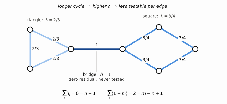
The picture above is the whole story on seven ligands. Every triangle edge has \(h = 2/3\), every square edge \(h = 3/4\), and the bridge \(h = 1\). Cycle length is what sets leverage, and one formula covers every case. Edge \(i\) is in parallel with everything else joining its endpoints, so writing \(r_i = \sigma_i^2\) for its own resistance and \(R_{\text{rest}}\) for that of the rest of the network,
\[h_i = \frac{R_{\text{rest}}}{r_i + R_{\text{rest}}}\]A bridge has no parallel path, \(R_{\text{rest}} = \infty\), so \(h = 1\). An edge lying in exactly one cycle of length \(\ell\) has the other \(\ell-1\) edges in series, so with unit weights \(h = (\ell-1)/\ell\) and \(1-h = 1/\ell\) — the triangle and the square above. An edge in several cycles has several paths in parallel and does better: the shared edge of two back-to-back triangles sees two 2-paths, \(R_{\text{rest}} = 1\), so \(h = 1/2\) rather than \(2/3\).
Each independent cycle contributes exactly one unit to the testability budget \(\sum_i(1-h_i)\), and a longer loop spreads that single unit over more edges. Redundancy is not free: closing a big loop tests each of its edges less than closing a small one.
a conserved budget of scrutiny
The leverages obey two sum rules that tie straight back to the subspace table:
\[\sum_i h_i = n - 1 \quad (\text{cut budget}), \qquad \sum_i (1 - h_i) = m - n + 1 \quad (\text{cycle budget})\]because \(\mathrm{tr}(\mathbf H) = \mathrm{rank}(\mathbf B)\). The first is Foster’s theorem in disguise. The two budgets behave quite differently, though. The cut budget \(n-1\) depends only on the number of ligands, so it is genuinely conserved: add an edge and the existing ones must give up leverage to make room — they compete for a fixed pool. The cycle budget \(m-n+1\) depends on the number of edges, so each edge you add raises it by exactly one. That is the precise version of “redundancy is what buys testability”: testability is created, not merely redistributed, and it is created one unit at a time.
deleting edges is a projection, not a restriction
The leave-one-out formula quietly did something worth pausing on: it refit. Why not just take the residual we already have and read off the entries for the edges that survived? Because the restriction of \(\tilde{\boldsymbol\epsilon}\) to a subgraph is NOT the subgraph’s residual, and it is not even a circulation on the subgraph.
Take an edge set \(S\) and delete some of its edges, leaving \(S'\) with \(k\) edges. A residual has to be a circulation on its own graph — that was the normal equations, \(\mathbf B_{S'}^\mathsf T\mathbf W_{S'}\tilde{\boldsymbol\epsilon}_{S'} = \mathbf 0\), Kirchhoff’s current law. Test the restricted vector against it and it fails, with an error you can write down exactly:
\[\mathbf B_{S'}^\mathsf T\mathbf W_{S'}\big(\tilde{\boldsymbol\epsilon}\big|_{S'}\big) = -\sum_{i\,\text{deleted}} w_i\,\tilde\epsilon_i\,\mathbf b_i \;\neq\; \mathbf 0\]The reading is physical. The full graph’s residual currents balanced at every node because every edge was there to carry them. Cut some edges and the current they were carrying has nowhere to go; what is left over piles up as divergence at the endpoints of whatever you removed. So the restricted vector sits outside the subgraph’s cycle space entirely, and the subgraph’s own residual is a genuinely new projection — which is why deleting one edge shifts the residual on every other edge, and why the leave-one-out formula needed Sherman–Morrison rather than an index lookup.
Two things do survive, and they are worth separating from what does not.
The cycle space nests. A loop lying entirely inside \(S'\) is still a loop of the full graph; pad its \(\pm 1\) vector with zeros and it is a full-graph circulation. So the subgraph’s cycle space is a genuine subspace of the original, of dimension \(k - n + 1\) instead of \(m - n + 1\). Deleting an edge that lies in a cycle costs exactly one independent loop.
Individual closure values do not move at all. For a loop \(\mathbf z\) inside \(S'\), the closure is \(\mathbf z^\mathsf T\mathbf y\) — a function of the data, not of any fit — so it reads the same before deletion, after deletion, and after refitting. The residual vector is fit-dependent and changes; the loop sums are not and do not.
That first point is the one to carry forward. Every deletion of a cycle edge shrinks the cycle space by one dimension, and there is a floor at zero.
never make closure the objective
Here is the trap the machinery above sets, and it is worth spelling out because it is an easy and expensive mistake.
Closure error is blind — computable with no experimental data — so it is tempting to optimize it: drop the edges that close worst, and the graph gets better. The reasoning is exactly backwards, and one line of algebra shows why.
Deleting an edge removes one non-negative term from the objective \(\sum_i w_i(y_i - \mathbf b_i^\mathsf T\mathbf x)^2\), and the surviving fit is free to re-optimize over the rest. So the minimum can only go down:
\[\chi^2_{S'} \;\le\; \chi^2_{S} \qquad \text{whenever } S' \subset S, \qquad \chi^2_{S} \equiv \min_{\mathbf x}\sum_{i\in S} w_i\,(y_i - \mathbf b_i^\mathsf T\mathbf x)^2\]Closure error is monotone non-increasing under edge deletion. It is not a quality score at all — it is a count of how much redundancy you have left. (It must be the weighted misfit, since that is what is being minimized; the plain \(\|\tilde{\boldsymbol\epsilon}\|\) of a weighted fit need not shrink, because the fit is not trying to make it small. Under OLS the two coincide.) And that immediately gives the global optimum: keep deleting until \(m = n-1\), a spanning tree, where the cycle space has dimension \(m-n+1 = 0\) and the residual is identically zero. A perfect score, though on the worst graph in the family. A tree has no redundancy, no cross-checks, and no way to average down noise — each \(\Delta G\) hangs on a single unverified chain of measurements. Minimizing closure error does not select good edges; it destroys the evidence that any edge was ever tested.
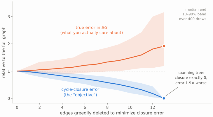
The figure runs the experiment on a 12-ligand graph with 24 edges, deleting the edge that most reduces closure error at each step, over 400 independent noise draws on the same graph and the same true \(\Delta G\)’s. Lines are medians, bands the 10th to 90th percentile. The blind objective falls in every single draw — it is the monotonicity result above — and reaches exactly zero at the spanning tree. The true error, invisible to the procedure, climbs the whole way and ends \(1.9\times\) worse at the median. The bands are the point: at the tree the 10th percentile of the true error is still \(1.19\), so even the luckiest draws come out behind, and \(97\%\) of them do. Note that nothing pathological was needed: the noise here is honest, independent, and identically distributed, exactly the OLS model of case 1. The degeneracy is structural, not a quirk of bad data.
This does not make closure useless; it makes it a diagnostic, never an objective. The quantities that survive optimization pressure are the ones normalized by how much testing the edge actually received: the held-out gap \(g_i\), the standardized residual, and \(\chi^2/\mathrm{dof}\), which divides by the very degrees of freedom that deletion destroys. A useful rule of thumb: if your objective can be improved by discarding data, it is measuring your data volume, not your data quality.
what closure cannot see
Both cases above assumed the errors are centered, \(\mathbb E[\boldsymbol\epsilon] = \mathbf 0\). For RBFE data this is almost certainly false, and the failure mode is systematic: if the force field misplaces one ligand’s free energy, every edge touching that ligand is wrong together.
Model this with a fixed per-ligand bias \(\boldsymbol\delta\in\mathbb R^n\):
\[\boldsymbol\epsilon = \mathbf B\boldsymbol\delta + \boldsymbol\eta\]where \(\boldsymbol\eta\) is the honest per-edge noise. The bias term is cycle-consistent by construction — it is a difference of node quantities — so it lies in \(\mathrm{col}(\mathbf B)\), and every closure quantity annihilates it:
\[\mathbf z^\mathsf T(\mathbf B\boldsymbol\delta) = \mathbf 0, \qquad (\mathbf I - \mathbf H)\,\mathbf B\boldsymbol\delta = \mathbf 0\]Meanwhile the estimate swallows it whole:
\[\hat{\mathbf x} - \mathbf x = \boldsymbol\delta + \mathbf L^{+}\mathbf B^\mathsf T\mathbf W\boldsymbol\eta \qquad (\text{up to the gauge, as always})\]The bias passes through one-for-one, unattenuated, while \(\chi^2\), every loop sum, and every residual do not move at all. One can corrupt the answer with 2 kcal/mol of per-ligand bias, and the closure diagnostics register nothing. On real RBFE data this decomposition can be fitted directly: regress the signed edge errors on \(\mathbf B\) and read off how the error splits between the cycle-consistent part \(\mathbf B\boldsymbol\delta\) and the rest. It is worth doing on your own data, because whatever that first fraction turns out to be is exactly the fraction no closure test can ever see.
Two corollaries close the loop, so to speak:
- ”\(\chi^2\) looks fine” is not evidence the free energies are good. It is evidence the cycle-visible noise matches the error bars — nothing more.
- Adding redundant edges does not help with bias. Extra cycles average down \(\boldsymbol\eta\) (that is the effective-resistance story), but \(\boldsymbol\delta\) rides through any topology, any weighting, any pruning of edges. Against ligand-level bias, the only remedies are better physics or external reference data.
summary
- Write the graph measurement problem as \(\mathbf y = \mathbf B\mathbf x + \boldsymbol\epsilon\). Two subspaces of \(\mathbb R^m\) do all the work: \(\mathrm{col}(\mathbf B)\) (dimension \(n-1\)), where the signal lives, and the cycle space (dimension \(m-n+1\)), where closure lives.
- \(\mathrm{Cov}(\hat{\mathbf x})\) is a sandwich \(\mathbf L^{+}\mathbf B^\mathsf T\mathbf W\boldsymbol\Sigma\mathbf W\mathbf B\mathbf L^{+}\) in general; it collapses to \(\sigma^2\mathbf L^{+}\) under OLS with iid noise and to \(\mathbf L^{+}\) under WLS with \(\mathbf W=\boldsymbol\Sigma^{-1}\), where variances of differences are effective resistances.
- Cycle closure and residuals are projections onto the cycle space (its \(\mathbf W\)-weighted analog under WLS). They see the cycle-inconsistent part of the error, calibrate error bars via \(\chi^2/(m-n+1)\), and are exactly blind to any cycle-consistent error — in particular per-ligand bias, which is typically the dominant term.
Cycle closure is a test of self-consistency, not of accuracy. It is well worth running — it is free, and, read through the held-out gaps rather than the raw residuals, it catches bad edges and dishonest error bars. Just do not read a clean closure as a clean calculation.
appendix: try it yourself
Everything above is about twenty lines of NumPy. This builds a graph, fits it, and prints the leverages, the two sum rules, the closure of a loop, and a brute-force check that the held-out formula is exact:
import numpy as np

# triangle 0-1-2, square 3-4-5-6, joined by a bridge 2-3
edges = [(0,1),(1,2),(2,0),(2,3),(3,4),(4,5),(5,6),(6,3)]
n, m  = 7, len(edges)

B = np.zeros((m, n))                      # signed incidence matrix
for i, (a, b) in enumerate(edges):
    B[i, a], B[i, b] = -1, +1

w  = np.ones(m)                           # w = 1/sigma^2 per edge; OLS here
W  = np.diag(w)
L  = B.T @ W @ B                          # graph Laplacian, = D - A
Lp = np.linalg.pinv(L)                    # singular: the global-offset gauge
H  = B @ Lp @ B.T @ W                     # hat matrix
h  = np.diag(H)                           # leverage per edge

print("h            ", h.round(3))                  # bridge is 1.0
print("sum h        ", h.sum(), " = n - 1 =", n-1)
print("sum (1-h)    ", (1-h).sum(), " = m - n + 1 =", m-n+1)

x = np.random.default_rng(0).normal(size=n)         # true per-ligand dG
y = B @ x + np.random.default_rng(1).normal(0, .3, m)
xh  = Lp @ B.T @ W @ y                              # the fit
eps = y - B @ xh                                    # closure residual

print("residual     ", eps.round(6))                # bridge entry is 0

z = np.zeros(m); z[[0,1,2]] = 1                     # the triangle loop
print("loop sum of y", z @ y, "== of residual", z @ eps)   # identical

i = 4                                               # held-out check, edge 4
keep = [j for j in range(m) if j != i]
Bk, yk, Wk = B[keep], y[keep], np.diag(w[keep])
xk = np.linalg.pinv(Bk.T @ Wk @ Bk) @ Bk.T @ Wk @ yk
print("refit gap    ", y[i] - B[i] @ xk)
print("closed form  ", eps[i] / (1 - h[i]))         # same to machine precision
Watch two things in the output. The bridge’s leverage is exactly
\(1\) and its residual exactly \(0\), and the two sum rules land on the integers
\(n-1\) and \(m-n+1\) no matter what weights you put in w — they are properties
of the graph, not of the data.


