Transcranial magnetic stimulation

This is a note I wrote while doing a project on transcranial magnetic stimulation coil design. TMS is an FDA approved treatment for depression.

introduction

Transcranial magnetic stimulation (TMS) is a non-invasive method to stimulate the nervous system. A current change in the stimulator circuit positioned near the brain cortex induces change in magnetic field in space and the latter then induces a change in the electric field in brain tissue. As a result, axonal membrane potential is changed and the functional areas of the brain cortex is stimulated. The induced field typically reaches no more than a few centimeters into the brain, i.e., it is a `shallow’ brain stimulation technique.

In a conventional (biphasic) TMS design, a capacitor is first charged to several \(kV\), and then discharged through the gating of a thyristor in a RCL oscillator circuit, generating a current of several \(kA\) in the coil in about \(100\mu s\), with a profile of a damped cosine shape. The peak magnetic field achieved near the coil can reach as big as \(4T\) and the induced magnetic field typically lasts for \(300\mu s\). A new generation of controllable TMS (cTMS) provides near-rectangular pulse shape, adjustable pulse width, number of phases and directionality parameters.

The induced electric field is known to be more effective in stimulating axons and dendrites if its direction is parallel to the neuronal structures. Most studies have been performed on the primary motor cortex (M1) where a focal muscle twitch can be produced, known as the motor-evoked potential (MEP).

TMS equipment that delivers stimuli with a repetition rate lower than \(1Hz\) are called single-pulse devices. They are mostly used in basic research studies where good temporal resolution is essential. Devices to deliver repetitive TMS pulses (\(1-50Hz\)) are also available, known as rTMS. It can produce lasting effects outside the stimulation period, sometimes known as `momentary lesions’ in the cerebral cortex. In general, trains of stimuli applied at low frequency (\(0.2-1Hz\)) inhibit neural activity while the ones applied at high frequency (\(5-20Hz\)) increase neural activity. Besides its role in studying brain physiology, TMS is also used clinically with applications in detecting demyelination, detecting stroke, improving motor function of patients with Parkinson’s disease, dystonia, stroke,
and reducing depression.

Comparing to the methods with electric stimulations such as transcranial electric stimulation (TES), its advantages include:

• It is largely a painless technique;
• The induced electric field is less sensitive to anatomical differences among subjects;
• The latency of TMS response is slightly shorter than TES.

Besides the known adverse effect of TMS such as seizure induction and mild headache, the disadvantages of TMS include:

• The high coil voltage/currents needed for neural stimulation requires bulky and costly devices;
• The stimulation precision is low;
• Only a pulsed electric field is generated and high repetition rate is difficult to achieve.

hardware design

The circuit of a biphasic TMS design is basically a RCL circuit with two nonlinear components: the thyristor S and diode D to avoid reverse charging.

Due to the large currents running through the wire and the resulting repulsive coil Lorentz force, the mechanical integrity of the coil needs to be carefully considered.

framework of calculation

the simplified brain model

For simplicity, we model brain tissue as linear, isotropic and homogeneous medium with electric conductivity \(\sigma\), electric permittivity \(\varepsilon\), and magnetic permeability \(\mu=\mu_0=4\pi\times10^{-7}Hm^{-1}\). The linearity assumption allows one to use the linear constitutive relation and Ohm’s law,

\[\begin{align} \mathbf D =& \varepsilon \mathbf E \\ \mathbf H = & \mathbf B / \mu_0 \\ \mathbf J = & \sigma \mathbf E. \end{align}\]

The isotropy assumption allows the scalar description of \(\varepsilon\), \(\mu\) and \(\sigma\) as in general they can be tensors under the linearity constraint. The homogeneity assumption further simplifies \(\varepsilon\), \(\mu_0\) and \(\sigma\) as three scalar numbers to describe the whole brain. Here we have assumed that the magnetic permeability of the brain is approximately equal to the vacuum value \(\mu_0\).

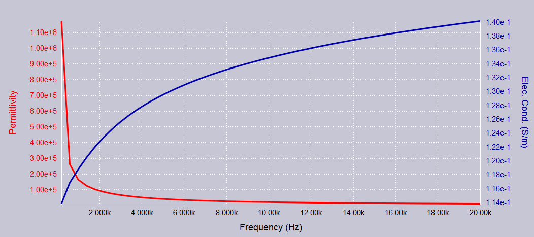
The frequency dependence of \(\sigma\) and \(\varepsilon\) of the brain (including both WM and GM) is shown in Fig. 1.

Fig. 1 Frequency dependence of the brain tissue dielectric properties \(\sigma\) and \(\varepsilon\). The permittivity is in the unit of \(\varepsilon_0\simeq8.85\times10^{-12}Fm^{-1}\). Data is acquired from the ITIS foundation. }

There are two dimensionless parameters that are of vital importance in characterizing the electro-magnetic (EM) response of a biological tissue \cite{Plonsey1967}: \(|k|R_{\max}\) and \(\omega\varepsilon/\sigma\), where \(R_{\max}\) is the maximal dimension of the sample, \(\omega\) and \(k\) are the angular frequency and the complex wave number of the induced EM wave.

The first parameter characterizes the wave propagation effect as \(|k|R_{\max}\) is the phase variation of the EM wave in the range of the sample. For reasons that would be clear later, the first and second parameters also controls the size of the inductive and capacitive properties of the sample respectively \cite{Plonsey1967}.

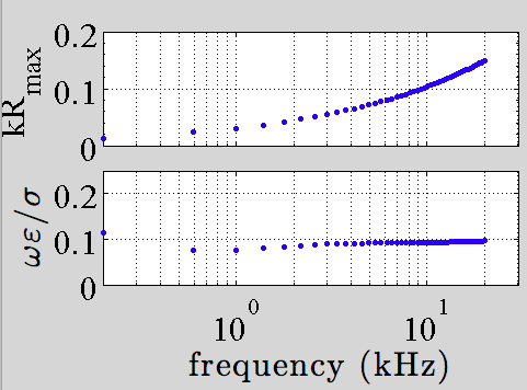
Assuming \(R_{\max}=1m\), we plot the two characteristic parameters of brain tissue in Fig. 2. Note in this wide frequency range, \(\omega\varepsilon/\sigma\) is small compare to \(1\).

Fig. 2 Frequency dependence of the two characteristic parameters of brain tissue. \(R_{\max}=1m\) is assumed.

quasi-static approximation

To get the equations for the induced electric field, we take the curl of the Maxwell-Faraday equation, plug in the previous Eq.s and use the fact that no free charge exists inside the homogeneous conductor, i.e., \(\nabla\cdot \mathbf E=0\). The end result is a damped wave equation

\begin{align} \nabla^2 \mathbf E = \mu_0\sigma\partial_t\mathbf E +\mu_0\varepsilon\partial_t^2\mathbf E. \end{align}

Carrying out harmonic analysis on \(\mathbf E\), i.e.,

\begin{align} \mathbf E = \mathbf E_0 e^{i(\omega t - \mathbf k\cdot \mathbf r)}, \end{align} we get the dispersion relation of a conductor \begin{align} k^2 = \omega\mu_0\sigma\left(\frac{\omega\varepsilon}{\sigma}-i\right). \end{align}

An insulator (\(\sigma\rightarrow 0\)) results in linear dispersion relation \(\omega = k{c}/{n}\), where \(c\) is the speed of light and \(n=\sqrt{\varepsilon/\varepsilon_0}\) is the refractive index. A conductor (\(\sigma\rightarrow\infty\)) results in De Broglie’s dispersion relation \begin{align} k = \sqrt{\frac{\mu_0\omega\sigma}{2}}\left(1-i \right). \end{align} The imaginary part of \(k\) characterizes the skin (penetration) depth \begin{align} \delta = \sqrt{2}/|k|=\sqrt{\frac{2}{\mu_0\omega\sigma}}. \end{align}

In general, the computation of the induced electric field inside a conductor is complicated since the wave propagation, the capacitive effect and the inductive effect are all present. The quasi-static approximation simplifies the calculation dramatically and it applies when the two characteristic parameters are small, i.e.,

\[\begin{align} |k|R_{\max}\ll &1 \\ \omega\varepsilon/\sigma\ll &1. \end{align}\]

In this approximation, the wave propagation effects, the capacitance effects and the inductive effects in the biological tissue can all be neglected. In other words, the tissue behaves as a standard conductor with instantaneous response \cite{Jackson1998}.

For brain tissue, the quasi-static approximation holds up to \(MHz\) , if the region of interest (\(R_{\max}\)) is of the order \(10cm\), as seen in Fig. 2. Also, the skin depth is easily beyond the \(10cm\) range. Note that a large skin depth does not guarantee the feasibility of deep brain stimulation as it is only a relative intensity measure.

The electric field induced in the TMS experiment contains two contributions \begin{align} \mathbf E =-\partial_t{\mathbf A} -\nabla\varphi= \mathbf E_{\mathbf A} + \mathbf E_{\varphi}, \end{align} where \(\mathbf E_{\mathbf A}\) is the induced electric field due to the time-varying magnetic field (Faraday’s law) and \(\mathbf E_\varphi\) is the field due to the accumulated electric charge on the tissue boundary. \(\mathbf A\) is the vector potential defined from \(\mathbf B = \nabla\times \mathbf A\), and \(\varphi\) is the scalar (electrostatic) potential associated with the boundary conditions.

electric field due to time-varying magnetic field

In the absence of brain tissue, the electric field generated by TMS coil can be computed with the quasi-static approximation \cite{Plonsey1967} \begin{align} \mathbf E_{\mathbf A} (\mathbf r , t) =-\partial_t\mathbf A= \frac{\mu_0}{4\pi} \int \frac{-\partial_t\mathbf j(\mathbf r’ , t)} {|\mathbf r - \mathbf r ‘ |}d^3 r’. \label{eq:basic} \end{align} \(\mathbf E_{\mathbf A}\) is a direct result of changing magnetic field from the coil and is thus known as the primary field \cite{Ilmoniemi1999}.

Note this Eq. enjoys two features that greatly facilitate analytical calculation. Firstly, \(\mathbf E\) has instantaneous temporal response with respect to \(\partial_t\mathbf j\). Thus we can drop the temporal dependence in the calculation, i.e., the inductive effect can be neglected. Secondly, the Cartesian components of \(\mathbf E\) along different axes decouple thus can be calculated separately.

This Eq. can be written in the differential form \begin{align} \nabla^2\mathbf E_{\mathbf A} = \mu_0 \partial_t\mathbf j. \end{align} Since only regions outside the wires are of interest,
\(\mathbf E_{\mathbf A}\) satisfies Laplace’s Equation. Suppose the wires are in the upper half space, then we are only interested in the field in the lower half space \(z<0\). The problem can then be formulated as a boundary value problem

\[\begin{align} \begin{cases} \nabla^2\mathbf E_{\mathbf A} = 0 \\ \mathbf E_{\mathbf A} (z=0) = \mathbf E_0, \quad \text{at } \partial \Omega \end{cases} \end{align}\]

where \(\mathbf E_0\) is the boundary condition. Thus \(\mathbf E_{\mathbf A}\) can be solved either as an integration, or as a solution to Laplace’s equation.

From now on, we assume the currents in all wires have the same time derivative, i.e., \begin{align} \dot j_0 (t) = -\partial_t j(\mathbf r , t) . \end{align} In other words, the spacial dependence of \(\dot j_0(t)\) is eliminated. This quantity can be viewed as a pseudo-charge density.

electric field due to induced charge on the tissue boundary

When the brain tissue is placed inside the primary field \(\mathbf E_{\mathbf A}\), surface charges are induced at the brain boundary as a result of the conductance difference of the brain tissue and its surroundings and they give rise to secondary field \(\mathbf E_\varphi\). Under the quasi-static approximation, this charge accumulation can be considered as instantaneous, i.e., the capacitive (charging) effect can be neglected.

Under the quasi-static assumption, the electrical field due to surface charges can be written as \begin{align} E_\varphi = -\nabla\varphi = \frac{\nabla}{4\pi\sigma}\int \frac{\Sigma(\mathbf r’,t)} {|\mathbf r-\mathbf r’|} dS’, \label{eq:E_phi} \end{align} where \(\Sigma\) is the surface charge density at the brain tissue boundary.

The static condition \(\nabla\cdot \mathbf J=0\) requires the normal component of the current to be continuous at the tissue boundary. Since current cannot flow outside the tissue, we have \begin{align} \hat n\cdot(\mathbf E_{\mathbf A} + \mathbf E_{\varphi} ) = 0 \label{eq:bc} \end{align} on the brain tissue side, where \(\hat n\) is the normal direction of the tissue boundary.

Thus there are two approaches to solving \(\mathbf E_\varphi\). One is to solve the source integral equation and the surface charge density \(\Sigma\) can be computed using Gauss’ theorem \begin{align} \Sigma = (\varepsilon+\varepsilon_0) \mathbf E_\varphi \cdot \hat n. \end{align}

The other approach is to solve \(\mathbf E_{\mathbf A}\) first, thus obtaining the boundary condition of \(\mathbf E_\varphi\) at the boundary, and then solve the differential equation \begin{align} \nabla\times \mathbf E_\varphi = 0 \quad \text{or} \quad \nabla\cdot\mathbf E_\varphi = 0 \end{align} which can be combined into Laplace’s equation

\[\begin{align} \begin{cases} \nabla^2\mathbf E_\varphi = 0 \\ \hat n \cdot \mathbf E_\varphi = -\hat n \cdot \mathbf E_{\mathbf A} \quad \text{at } \partial\Omega. \end{cases} \end{align}\]